Logistic Regression parameters

Overview:

In the ever-evolving landscape of machine learning, the ability to seamlessly create, train, and evaluate models is crucial for both novice and expert data scientists. OtasML stands out as a visual machine-learning tool designed to simplify these processes, enabling users to interact intuitively with complex algorithms and configurations. In this article, we delve into the intricacies of logistic regression within OtasML, exploring its various settings and how they can be fine-tuned for optimal performance.

Configurations page:

The Configurations page is where the magic happens. Here, users can adjust a myriad of parameters that govern the behavior and performance of logistic regression models. Let's explore these parameters in detail:

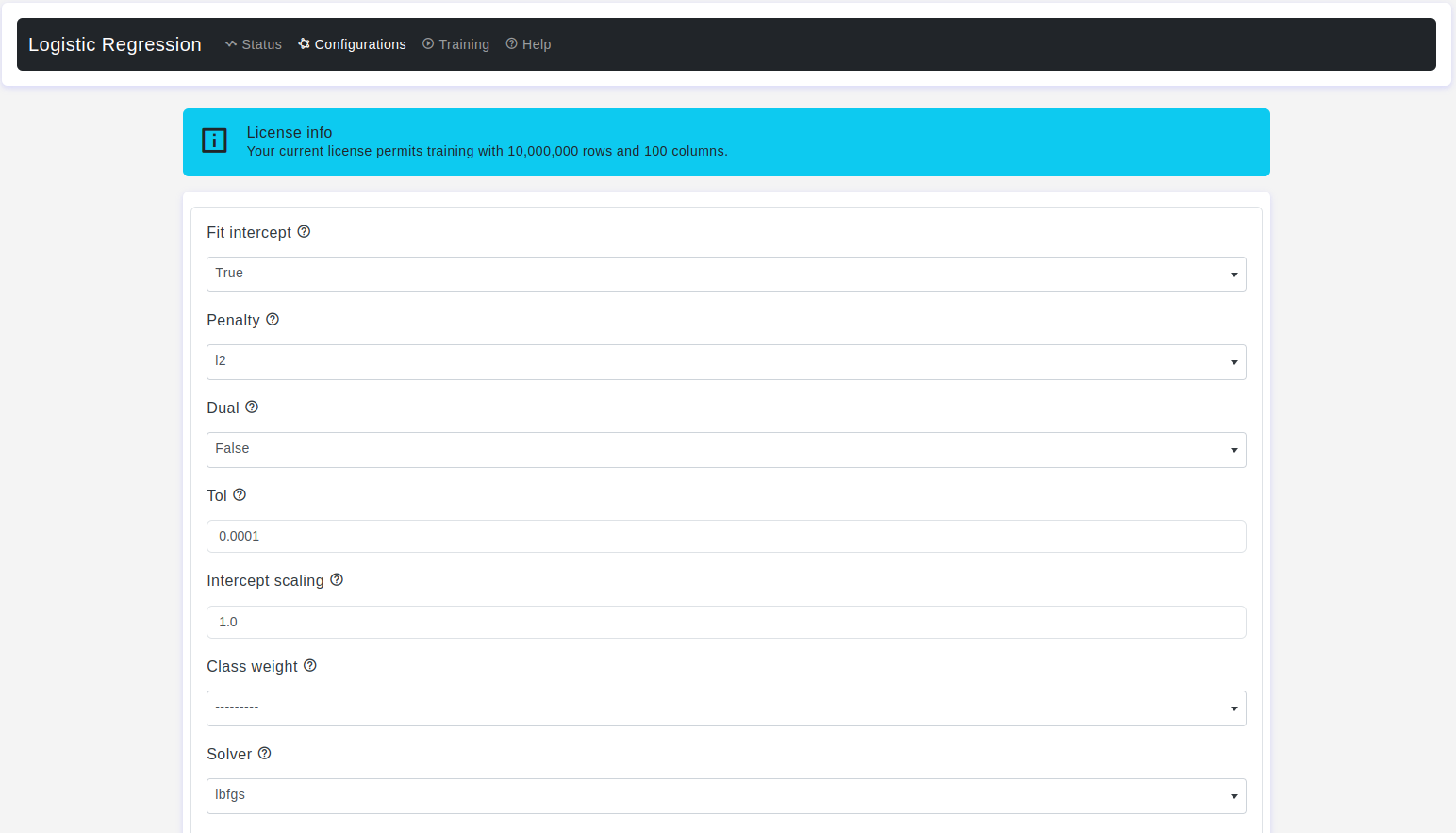
Fit Intercept

• Default Value: True
• Description: This parameter determines whether the model should include an intercept term in the decision boundary equation. The intercept term represents the predicted log-odds when all input features are zero.

Penalty

• Default Value: l2
• Description: Specifies how the data should be aggregated and represented within each cell of the histogram-like grid that forms the basis of the density contour plot. It allows you to choose a function that calculates a summary value based on the data points falling within each cell. Options include:
  • l1: Adds an L1 penalty term.
  • l2: Adds an L2 penalty term (default).
  • elasticnet: Combines both L1 and L2 penalties.
  • None: No penalty is added.

Dual

• Default Value: False
• Description: It is a concept that applies to the optimization problem associated with solving the logistic regression model. It is used to indicate whether the primal or dual optimization problem should be solved.
• Warning: Dual formulation is only implemented for l2 penalty with liblinear solver.

Tol

• Default Value: 1e-4
• Description: The tolerance for stopping criteria, which dictates when the optimization process should cease.

Intercept Scaling

• Default Value: 1.0
• Description: Refers to a technique used to handle regularization of the intercept term (also known as the bias term) in the logistic regression model. Regularization is a method to prevent overfitting by adding a penalty term to the loss function, which discourages overly complex models. Useful only when the solver liblinear is used and fit intercept is set to True.

Class Weight

• Default Value: None
• Description: Refers to assigning different weights to different classes within a binary classification problem. Logistic regression aims to find a decision boundary that separates two classes based on input features, and if not given, all classes are supposed to have weight one. Options include:
  • None: All classes have weight one.
  • Balanced: Adjusts weights inversely proportional to class frequencies.

Solver

• Default Value: lbfgs
• Description: It is an optimization algorithm that is used to find the optimal values of the coefficients (weights) of the features in the logistic regression model. These coefficients determine the relationship between the input features and the predicted log-odds (also known as the linear decision boundary) of the binary outcome.. Available solvers include:
  • lbfgs: Suitable for large datasets.
  • liblinear: Ideal for small to medium datasets.
  • newton-cg: Effective for multiclass classification.
  • newton-cholesky: Limited to binary classification.
  • sag: Suitable for large datasets with fast convergence.
  • saga: Extension of sag, supports both L1 and L2 regularization.

• Warning: The choice of the algorithm depends on the penalty chosen. Supported penalties by solver:

  • lbfgs [l2, None]
  • liblinear [l1, l2]
  • newton-cg [l2, None]
  • newton-cholesky [l2, None]
  • sag [l2, None]
  • saga [elasticnet, l1, l2, None]

Max Iter

• Default Value: 100
• Description: The maximum number of iterations for the solver.

Multi Class

• Default Value: auto
• Description: Determines how to handle multi-class classification. Options include:
  • auto: auto Selects ovr if the data is binary, or if solver=liblinear, and otherwise selects multinomial.
  • ovr: In this approach, you train a separate binary logistic regression model for each class while treating the other classes as a single combined class. For example, if you have classes A, B, and C, you would create three binary logistic regression models: A vs. (B and C), B vs. (A and C), and C vs. (A and B). During prediction, each model produces a probability score, and the class with the highest probability is chosen as the predicted class.
  • multinomial: This is a direct extension of binary logistic regression to multi-class problems. Instead of training separate models, you train a single model with multiple output classes. The Multinomial function is applied to the output of each class, converting the scores into probabilities that sum up to 1. During prediction, the class with the highest probability is selected as the predicted class..

Verbose

• Default Value: 0
• Description: It is a parameter that controls the amount of information displayed during the training process. It determines whether or not the algorithm provides additional output or logging while it's iterating to find the optimal coefficients for the logistic regression model. The verbose parameter is typically used for debugging and monitoring purposes to understand the progress of the optimization process and gather insights about how the algorithm is performing.
• Warning: For the liblinear and lbfgs solvers set verbose to any positive number for verbosity.

Warm Start

• Default Value: False
• Description: It is a feature that allows you to initialize the coefficients of the logistic regression model with the solution from a previous model. It's a technique used to speed up the convergence of the optimization process, especially when you're iteratively fitting the same model to different subsets of data or making incremental adjustments to the model's parameters. When the warm start is True, the coefficients obtained from a previous fit serve as a starting point for the optimization process on the current dataset. This can lead to faster convergence and potentially fewer iterations needed to find the optimal solution.

N Jobs

• Default Value: None
• Description: It refers to the number of CPU cores or parallel processes that can be utilized to perform computations in parallel. It's a parameter that controls the parallelism of certain operations during the training or prediction process. Parallelism can significantly speed up the execution of computationally intensive tasks, such as fitting a model on a large dataset or making predictions on a large number of samples. By leveraging multiple CPU cores, you can distribute the workload and process data more quickly.
• Warning: A number of CPU cores are used when parallelizing over classes if multi_class= ovr. This parameter is ignored when the solver is set to liblinear regardless of whether multi_class is specified or not. -1 means using all processors.

L1 Ratio

• Default Value: None
• Description: It refers to a parameter that determines the balance between L1 and L2 regularization in the model. L1 and L2 regularization are techniques used to prevent overfitting by adding penalty terms to the loss function, discouraging overly complex models.
• Warning: With 0 <= l1_ratio <= 1. Only used if penalty=elasticnet. Setting l1_ratio=0 is equivalent to using penalty='l2', while setting l1_ratio=1 is equivalent to using penalty='l1'. For 0 < l1_ratio <1, the penalty is a combination of L1 and L2.

Random State

• Default Value: None
• Description: It is a parameter that allows you to control the random number generator used for various random processes during the training and evaluation of the model. These random processes can include initializing the model's coefficients, shuffling the dataset, or splitting the data into training and testing subsets.
• Warning: Used when solver = sag, saga or liblinear to shuffle the data.

C

• Default Value: 1.0
• Description: It is a regularization hyperparameter that controls the strength of regularization applied to the model's coefficients. Regularization is a technique used to prevent overfitting by adding a penalty term to the loss function, which discourages overly complex models.
• Warning: must be a positive float.

Test Size

• Default Value: 0.2
• Description: The test size parameter is used when splitting the dataset into these subsets, and it specifies the portion of the data that will be used for testing.

Train Size

• Default Value: 0.8
• Description: The train size parameter is used when splitting the dataset into these subsets, and it specifies the portion of the data that will be used for model training.

Conclusion

OtasML provides a robust and user-friendly interface for configuring logistic regression models. By understanding and leveraging the detailed configurations available, users can fine-tune their models to achieve the best performance on their datasets. Whether you are balancing class weights, choosing the right solver, or setting the appropriate regularization, OtasML empowers you to make informed decisions with ease. Dive into OtasML today and harness the power of visual machine learning to elevate your data science projects.